Microarray Analysis for DEGs

Microarray Analysis for Differential Gene Expression: A Case Study on SARS Using GEO NCBI 

There are almost 24000 genes that are encoded by human genome. These genes do not make different types of proteins all the time. So to understand which gene is going to make which protein product under which conditions we study the expression of genes. Microarray analysis is the most commonly used method to analyze the gene expressions in human body.

Microarray Methodology: 

Microarray is a tool used to analyze thousands of gene expression at a time. There are several key steps that are followed for microarray analysis:

1. Sample Isolation, the RNA is extracted from both malignant and healthy sample is extracted and then isolated. 
2. RNA extraction and isolation is done in stringent conditions because RNA is highly unstable and we use dry ice for it. 
3. RNA is then converted into cDNA using reverse transcriptase PCR and adding Oligo DTs which is relatively stable molecule. Oligo DTs, which are only thymine nucleotides are added because of Poly-A tail (a post-transcriptional modification).
4. The cDNA is then fluorescently labelled with different colors, for instance the malignant sample with yellow and healthy sample with green.
5. Thousands of spots having DNA probes, which are short oligonucleotides that cover the sequence of specific gene, are placed over microarray chip. 
6. The laser excites the flourescent dye and the emission levels are measured by a detector.
7. And the results of microarray analysis are checked by using GEO NCBI.

 Here in this blog we will take an example of respiratory disease SARS and how the results can be analyzed by using bioinformatics tools GEO NCBI and geo2r. 

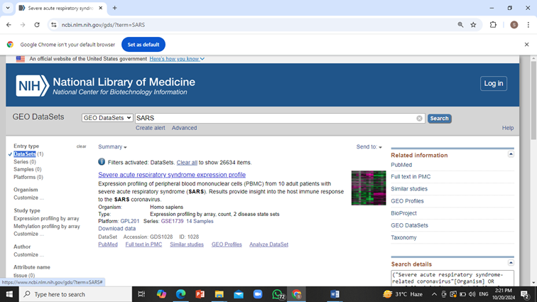
1. First open NCBI and write SARS in the search bar and select GEO datasets from drop down menu and click on search.

   

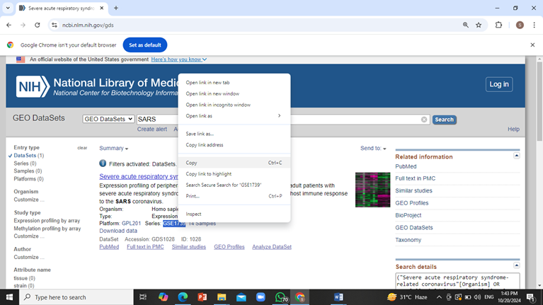
2. From the side bar select ‘Datasets’ and copy the series accession number i.e. GSE1739 in case of SARS. 

   

   

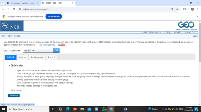
3. Go to GEO2R website and paste the accession number in the search bar and click on ‘Set’.  

   

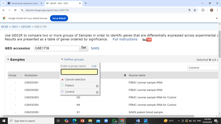
4. Now create two groups i.e. ‘Patient’ and ‘Control’ by clicking on “Define Groups” option and sort the resulting samples into their respective groups (select all the control sample and click on control group and then select the patient samples and click on patient group).

   

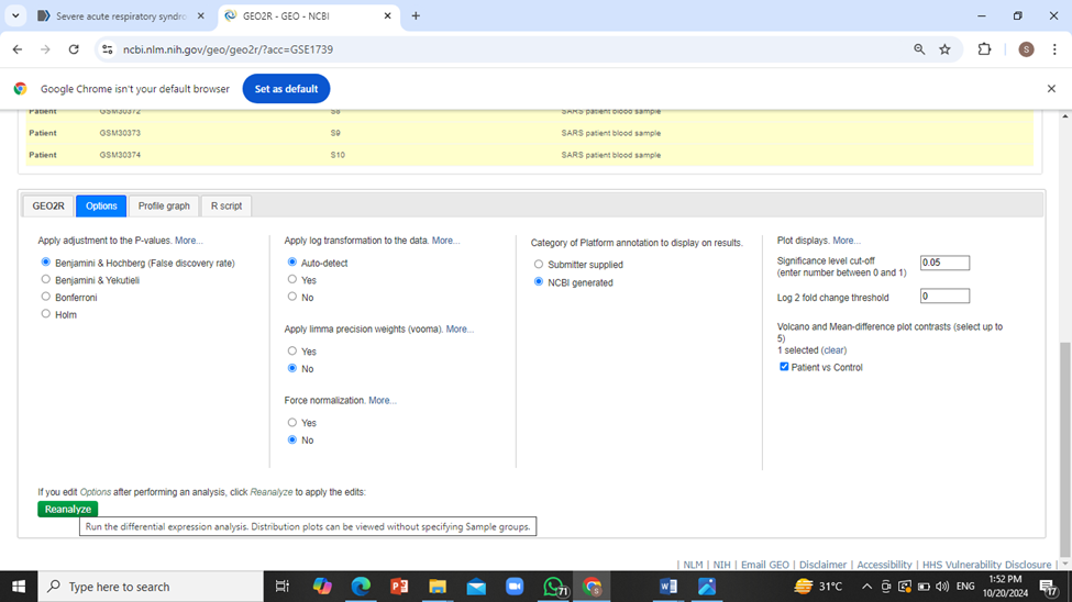
5. Scroll down and click on ‘Options’ tab, make sure to apply adjustments to the P-values as Benjamini and Hochberg (False Discovery Rate) and also click on Patient vs Control box and then click on ‘Reanalyze’.

   

    

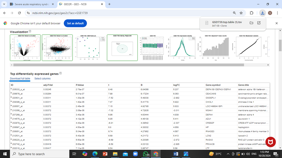
6. Now download the full table representing differentially expressed genes by click on ‘Download full table’.

   

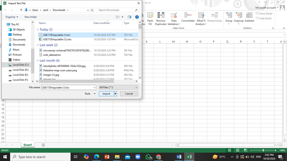
7. Open this table data in MS Excel file. For this purpose, select the following in excel: ‘data’ tab -> ‘From Text’ and then open the text file recently downloaded and load it into excel. 

   

   

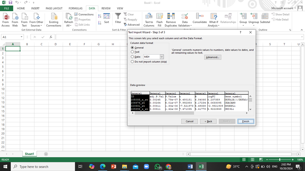
8. Click on ‘Next’ twice and then click on ‘Finish’. The data will be downloaded onto the excel sheet. 

   

   

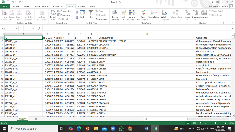
9. To narrow down this huge amount of data to only show those genes that have significant effects on patients, we will apply a filter to ‘adjusted P value’ column so that only genes with the P value less than or equal to 0.05 will be shown. 

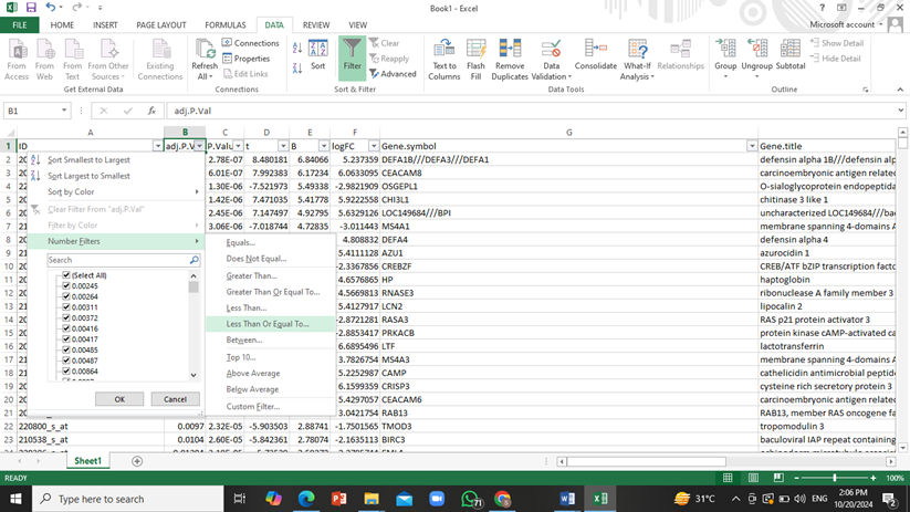
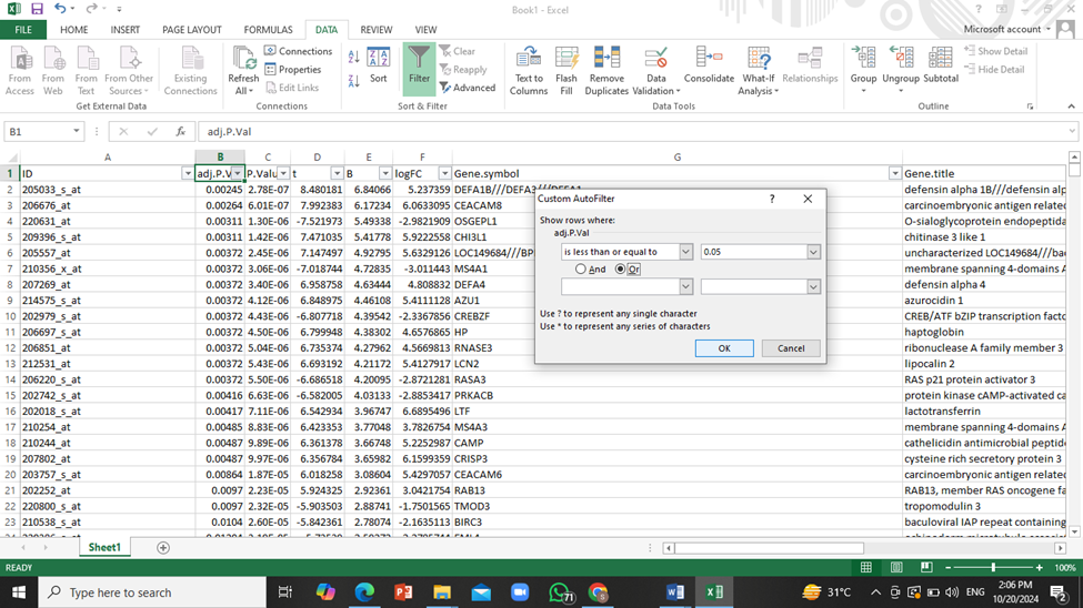
10. For this purpose go to DATA tab and click on ‘Filter’, then click on downwards arrow next to adjusted P value column and select the following: ‘number filter’ -> ‘less than or equals to’ and then enter ‘0.05’. 

    

    

    Interpretation:

    The P-value basically illustrates the statistical significance which tells about the probability of occurring an event. It’s threshold value should be 0.05 minimum. If the P-value is 0.05 or less then its significance increases. Adjusted P-value is more reliable and accurate then simple P-value.

    Log FC (Fourier Count) takes the difference of gene expression value in patient’s sample to control’s sample and then gives the algorithm of it. Those values of Log FC should be selected that are more than +1 and less than -1.   
    References:

    Shi, L., Shi, L., Reid, L. H., Jones, W. D., Shippy, R., Warrington, J. A., Baker, S. C., Collins, P. J., De Longueville, F., Kawasaki, E. S., Lee, K. Y., Luo, Y., Sun, Y. A., Willey, J. C., Setterquist, R. A., Fischer, G. M., Tong, W., Dragan, Y. P., Dix, D. J., . . . Slikker, W. (2006). The MicroArray Quality Control (MAQC) project shows inter- and intraplatform reproducibility of gene expression measurements. Nature Biotechnology, 24(9), 1151–1161. https://doi.org/10.1038/nbt1239     

    Edgar, R. (2002). Gene Expression Omnibus: NCBI gene expression and hybridization array data repository. Nucleic Acids Research, 30(1), 207–210. https://doi.org/10.1093/nar/30.1.207     

    Barrett T, Wilhite SE, Ledoux P, Evangelista C, Kim IF, Tomashevsky M, Marshall KA, Phillippy KH, Sherman PM, Holko M, Yefanov A, Lee H, Zhang N, Robertson CL, Serova N, Davis S, Soboleva A. NCBI GEO: archive for functional genomics data sets--update. Nucleic Acids Res. 2013 Jan;41(Database issue):D991-5. doi: 10.1093/nar/gks1193. Epub 2012 Nov 27. PMID: 23193258; PMCID: PMC3531084. https://pubmed.ncbi.nlm.nih.gov/23193258/     

    Alter, O., Brown, P. O., & Botstein, D. (2000). Singular value decomposition for genome-wide expression data processing and modeling. Proceedings of the National Academy of Sciences, 97(18), 10101–10106. https://doi.org/10.1073/pnas.97.18.10101